2025年12月28日日曜日

宇垣 隊


特別攻撃隊 戦没者名簿(準特攻:終戦後編)
宇垣特攻随行者
所属隊名階級氏名出身出身別生年戦死日享年乗機出撃基地戦死場所備考
第五航空艦隊司令長官中将宇垣 纏岡山海兵40期・海大22期18901945年8月15日56彗星大分沖縄方面中津留・遠藤機に同乗
第七〇一海軍航空隊大尉中津留 達雄大分海兵70期1945年8月15日彗星大分沖縄方面
第七〇一海軍航空隊飛曹長遠藤 秋章愛媛乙飛9期1945年8月15日彗星大分沖縄方面
第七〇一海軍航空隊中尉伊藤 幸彦宮城海兵73期1945年8月15日彗星大分沖縄方面
第七〇一海軍航空隊上飛曹大木 正夫福島乙飛17期1945年8月15日彗星大分沖縄方面
第七〇一海軍航空隊上飛曹山川 代夫山形丙飛(期不明)1945年8月15日彗星大分沖縄方面
第七〇一海軍航空隊中尉北見 武夫新潟海兵73期1945年8月15日彗星大分沖縄方面
第七〇一海軍航空隊中尉池田 武徳福岡予学13期1945年8月15日彗星大分沖縄方面
第七〇一海軍航空隊上飛曹山田 勇夫千葉甲飛11期1945年8月15日彗星大分沖縄方面
第七〇一海軍航空隊上飛曹渡辺 操千葉甲飛11期1945年8月15日彗星大分沖縄方面
第七〇一海軍航空隊中尉内海 進岩手予学13期1945年8月15日彗星大分沖縄方面
第七〇一海軍航空隊上飛曹後藤 高男福岡丙飛(期不明)1945年8月15日彗星大分沖縄方面
第七〇一海軍航空隊少尉磯村 堅山口予学(兵科)1期1945年8月15日彗星大分沖縄方面
第七〇一海軍航空隊二飛曹松永 茂男福岡特乙飛1期1945年8月15日彗星大分沖縄方面
第七〇一海軍航空隊一飛曹中島 英男愛知乙飛18期1945年8月15日彗星大分沖縄方面
第七〇一海軍航空隊一飛曹藤崎 孝良鹿児島丙飛(期不明)1945年8月15日彗星大分沖縄方面
第七〇一海軍航空隊一飛曹吉田 利滋賀乙飛18期1945年8月15日彗星大分沖縄方面
第七〇一海軍航空隊一飛曹日高 保鹿児島乙飛18期1945年8月15日彗星大分九州南方海域不時着により殉職
神州不滅特別攻撃隊
隊名階級氏名出身出身別生年戦死日享年乗機出撃基地戦死場所備考
神州不滅特別攻撃隊中尉今田 達夫広島幹候8期1945年8月19日九七戦大虎山南満東峰付近陸軍第五練習飛行隊第一教育隊大虎山分遣隊(満州派遣第一六六七五部隊)
神州不滅特別攻撃隊中尉馬場 伊与次山形幹候9期1945年8月19日九七戦大虎山南満東峰付近陸軍第五練習飛行隊第一教育隊大虎山分遣隊(満州派遣第一六六七五部隊)
神州不滅特別攻撃隊中尉岩佐 輝夫北海道特操1期1945年8月19日九七戦大虎山南満東峰付近陸軍第五練習飛行隊第一教育隊大虎山分遣隊(満州派遣第一六六七五部隊)
神州不滅特別攻撃隊中尉大倉 巌北海道特操1期1945年8月19日九七戦大虎山南満東峰付近陸軍第五練習飛行隊第一教育隊大虎山分遣隊(満州派遣第一六六七五部隊)
神州不滅特別攻撃隊中尉谷藤 徹夫青森特操1期1945年8月19日九七戦大虎山南満東峰付近陸軍第五練習飛行隊第一教育隊大虎山分遣隊(満州派遣第一六六七五部隊)
神州不滅特別攻撃隊中尉北島 幸次東京特操1期1945年8月19日九七戦大虎山南満東峰付近陸軍第五練習飛行隊第一教育隊大虎山分遣隊(満州派遣第一六六七五部隊)
神州不滅特別攻撃隊中尉宮野 進二東京特操1期1945年8月19日九七戦大虎山南満東峰付近陸軍第五練習飛行隊第一教育隊大虎山分遣隊(満州派遣第一六六七五部隊)
神州不滅特別攻撃隊中尉日野 敏一兵庫予下(期不明)1945年8月19日九七戦大虎山南満東峰付近陸軍第五練習飛行隊第一教育隊大虎山分遣隊(満州派遣第一六六七五部隊)
神州不滅特別攻撃隊中尉波多野 五男広島予下(期不明)1945年8月19日九七戦大虎山南満東峰付近陸軍第五練習飛行隊第一教育隊大虎山分遣隊(満州派遣第一六六七五部隊)
神州不滅特別攻撃隊少尉二ノ宮 清静岡少飛(期不明)1945年8月19日九七戦大虎山南満東峰付近陸軍第五練習飛行隊第一教育隊大虎山分遣隊(満州派遣第一六六七五部隊)
終戦直後に自決した待機特攻隊員
隊名階級氏名出身出身別生年戦死日享年乗機出撃基地自決場所自決状況
と号第二三〇部隊少尉河西 督郎特操2期1945年8月16日八日市琵琶湖竹生島沖飛行場離陸後、琵琶湖竹生島沖に突入自爆
第一六八振武隊中尉西川 俊彦陸士57期1945年8月18日八日市浅間山頂南斜面飛行場離陸後、長野県岩田村小学校に遺書投下、浅間山頂南斜面に自爆
第五十九振武隊少尉林 一男特操1期1945年8月18日都城東飛行場都城東飛行場の隊員宿舎裏手の山林にて自決
誠第一一六飛行隊軍曹栗城 良人少飛10期1945年8月20日朧潭飛行場台湾の朧潭飛行場で拳銃自決
回天神州隊大尉橋口 寛海兵72期1945年8月18日出撃予定の乗艇に第二種軍装で座り拳銃自決
特殊潜航艇(艦長)大尉畠中 和夫海兵72期終戦後に佐伯基地を出港し沖縄南下中操舵不能、乗員を帰投させ拳銃自決
第三十三突撃隊少尉松尾 秀輔海兵74期1945年8月25日大神基地練兵場甲板士官としての業務処理を終えた後、手榴弾自決

2025年12月20日土曜日

MATH LAB GPS PLUTO


https://jp.mathworks.com/help/satcom/ug/gps-receiver-acquisition-and-tracking-using-pluto-sdr.html   参照


GPS Signal Transmission, Acquisition and Tracking Using PlutoSDR

This example shows how to use an ADALM-PLUTO radio for over-the-air transmission and reception of a Global Positioning System (GPS) waveform generated using Satellite Communications Toolbox.

Introduction

In this example, you use an ADALM-PLUTO radio to perform over-the-air transmission of a composite GPS signal. To generate a composite GPS signal, follow these steps

  1. Get legacy GPS waveforms from multiple satellites. For more information about how to set the various parameters required to generate a GPS baseband waveform, see the GPS Waveform Generation example.

  2. Add Doppler shift and delay to each satellite waveform, and form the composite signal.

This ADALM-PLUTO radio transmits the GPS baseband waveform in repeat mode. The same ADALM-PLUTO radio can receive the transmitted GPS signal to perform acquisition, and track the code phase and carrier frequency of the satellites detected from the acquisition operation. The acquisition and tracking shown in this example are for GPS signals that contain coarse acquisition (C/A) codes. To set up the hardware, follow the instructions on the Installation and Setup page.

You can also explore the GPS Receiver Acquisition and Tracking Using C/A-Code example for a simulation example that does not require any hardware.

This figure outlines the process of GPS signal transmission and reception.

GPS_Pluto_SDR.png

This example consists of these sections.

  • Configure Simulation Parameters — Set various parameters to generate the waveform, and configure the GPS receiver.

  • Generate GPS Waveform — Generate GPS waveforms from multiple satellites, add delay, Doppler shift, and noise.

  • Configure PlutoSDR — Configure Pluto radio sample rate, center frequency, and other parameters for transmission and reception.

  • Acquisition and Tracking — Find the visible satellites and calculate coarse values of Doppler frequency offset and timing offset. Track the changing Doppler offset and code phase of the incoming signal.

Configure Simulation Parameters

Configure the simulation parameters by following these steps.

1. Set the control flag ShowVisualizations to true. This enables you to see all the output plots. Specify the number of GPS satellites to include in your waveform.

ShowVisualizations =  true;
% Transmitter Configuration
% Specify the number of GPS satellites in the waveform.
numSat = 4;

2. Specify the pseudorandom noise (PRN) identification numbers (ID) for the satellites visible to the receiver. The length of PRNIDs must be equal to or greater than the number of specified satellites numSat. If the length of PRINDs is greater than the value of numSat, this example considers only the first N elements of PRINDs for simulation, where N is the value of numSat.

PRNIDs = [2; 4; 11; 8]; 

3. Specify the number of data bits NumNavDataBits. Use the NumNavDataBits value to generate a GPS waveform for a specified number of data bits of navigation data. In general, the entire GPS legacy navigation data consists of 25 frames. Each frame comprises 1500 bits. This navigation data contains the ephemeris, clock, and almanac information. Because generating a waveform of this size can take a lot of time, this example generates the GPS waveform for a NumNavDataBits value of 200 bits.

% Set this value to control the number of navigation data bits in the
% generated waveform
NumNavDataBits = 200;

4. Set the bit starting index of the navigation data NavDataBitStartIndex. Use NavDataBitStartIndex to generate a GPS waveform from a random index of the navigation data.

NavDataBitStartIndex = 1321;

5. Set the sample rate at which to transmit GPS waveform.

SampleRate = 3.41e6;  % In samples/sec

6. Set the signal-delay values. Each satellite is a different distance from the GPS receiver. Therefore, the delay introduced on each signal is different for each satellite. Specify the number of C/A code chips delay for each satellite as a column vector. Delay values can be fractional because transmission time is not likely to be an integer multiple of the C/A code chip duration of 0.9775 microseconds.

sigdelay = [300.34; 587.21; 425.89; 312.88]; % Number of C/A code chips delay

7. Set the Doppler shift and Doppler rate. Because the velocity and position of each satellite is different, the Doppler shift and Doppler rate introduced for each satellite is also different. This example models Doppler shift as a sinusoidally varying frequency offset. For more information about latency and Doppler shift in a satellite scenario, see the Calculate Latency and Doppler in a Satellite Scenario example.

% Initialize peak Doppler shift and Doppler rate for each satellite. This example can track Doppler shift from -10KHz to 10KHz.
peakDoppler = [3589; 4256; 8596; 9568]; % In Hz
dopplerRate = [1000; 500; 700; 500];    % In Hz/sec

Receiver Configuration

To Configure the GPS receiver, set these parameters.

1. Set noise bandwidth for frequency-locked loops (FLLs), phase-locked loops (PLLs), and delay-locked loops (DLLs).

PLLNoiseBandwidth = 80; % In Hz
FLLNoiseBandwidth = 4;  % In Hz
DLLNoiseBandwidth = 1;  % In Hz

In GPS receivers, tracking algorithms track frequency, phase, and delay using frequency-locked loops (FLLs), phase-locked loops (PLLs), and delay-locked loops (DLLs), respectively. A wider loop bandwidth enables faster tracking, but can cause you to lose lock at low SNRs. A narrower loop bandwidth performs well at low SNRs, but tracks phase, frequency, and delay changes more slowly. For more information on interpreting these properties, see the Acquisition and Tracking section of this example.

2. Set the PLL integration time to 1 millisecond.

IntegrationTime = 1e-3; % In seconds

Generate GPS Waveform

A GPS waveform contains Precision-code (P-code) on the in-phase branch and C/A code on the quadrature-phase branch. In general, a GPS satellite transmits the waveform on the L1 frequency (1575.42 MHz). However, this example sets the transmitting frequency to 2.41 GHz to avoid interfering with real-time GPS signals. For more details about the GPS data generated in this example, see the IS-GPS-200 standard [1].

This example generates a GPS baseband waveform for each satellite, models the delay of each satellite signal independently, and combines all signals to generate the composite signal. Generate a GPS waveform by following these steps.

1. Set the number of extra navigation data bits for delay modeling numBitsForDelay. Setting numBitsForDelay to 1 introduces a maximum of 20 milliseconds into the signal. To introduce higher delay values, increase numBitsForDelay by an integer value.

numBitsForDelay = 1;

2. Create a HelperGPSNavigationConfig object to generate a legacy GPS waveform for each satellite. Each HelperGPSNavigationConfig object contains the information transmitted by a satellite. Because the focus of this example is explaining acquisition and tracking operations, rather than decoding data, this example keeps the parameters constant for all satellites.

%Initialize output waveform
resultsig = 0;

% Generate waveform from each satellite
for isat = 1:numSat
    % Create the legacy navigation (LNAV) configuration object
    lnavConfig = HelperGPSNavigationConfig("SignalType","LNAV","PRNID",PRNIDs(isat));

    % Generate the navigation data bits from the configuration object
    lnavData = HelperGPSNAVDataEncode(lnavConfig);

    % Configure the GPS waveform generation properties
    t = lnavConfig.HOWTOW*6; % First get the initial time
    % HOWTOW is an indication of the next subframe starting point. Because
    % each subframe is 300 bits long, you must subtract 300 bits from the
    % initial value to get the starting value of the first subframe. This
    % value can be negative as well. Because bit is of a 20 millisecond
    % duration, to get the time elapsed for bits, you must multiply the bit
    % index by 20e-3.
    bitDuration = 20e-3; % In sec
    pCodeRate = 10.23e6; % In Hz
    numPChipsPerNavBit = bitDuration*pCodeRate;
    navdatalen = length(lnavData);
    offsetTime = mod(NavDataBitStartIndex-301,navdatalen)*bitDuration;
    inittime = t + offsetTime;

    % To model delay, get one extra navigation bit from the previous bit
    navBitIndices = mod(NavDataBitStartIndex+(-1*numBitsForDelay:(NumNavDataBits-1)),navdatalen);
    navBitIndices(navBitIndices==0) = navdatalen;
    navbits = lnavData(navBitIndices);
    navdata = 1 - 2*navbits;
    upSampledNavData = repelem(navdata,numPChipsPerNavBit,1); 

    % Generate P-code and C/A code
    pgen = gpsPCode("PRNID",PRNIDs(isat),"InitialTime",inittime, ...
        "OutputCodeLength",(NumNavDataBits+numBitsForDelay)*numPChipsPerNavBit);
    pcode = 1 - 2*double(pgen());

    % Reduce the power of the I-branch signal by 3 dB, per IS-GPS-200 [1].
    % See table 3-Va in [1].
    isig = pcode/sqrt(2);

    cacode = 1 - 2*double(gnssCACode(PRNIDs(isat),"GPS"));

    numCACodeBlocks = (NumNavDataBits + numBitsForDelay)*bitDuration*1e3;
    caCodeBlocks = repmat(cacode(:),int64(numCACodeBlocks),1);

    % Because C/A code is 10 times slower than P-code, repeat each sample
    % of C/A code 10 times
    qsig = repelem(caCodeBlocks,10,1);

    % Generate the baseband waveform
    gpsBBWaveform = (isig + 1j*qsig).*upSampledNavData;

    % Initialize the number of samples per bit
    numSamplesPerBit = SampleRate*bitDuration;
    
    % Introduce Doppler
    numSamplesGPSBB = length(gpsBBWaveform);
    sampleIndices = (0:(numSamplesGPSBB-1));
    ph = sin(dopplerRate(isat)*sampleIndices/(peakDoppler(isat)*10.23e6));
    phase = 2*pi*(peakDoppler(isat)^2)/dopplerRate(isat)*ph;
    bbwave = gpsBBWaveform(:).*exp(1j*phase(:));

    % Rate match the generated signal to the radio sample rate
    [upfac,downfac] = rat(SampleRate/10.23e6);
    upgcode = repelem(bbwave,upfac,1);
    gpsWaveform = upgcode(1:downfac:end);

    % Get the number of samples for delay
    caCodeRate = 1.023e6;
    numDelaySamples = floor(sigdelay(isat)*SampleRate/caCodeRate);

    % Add delay to the signal by keeping samples of the previous bit at the
    % beginning of the signal
    delayedSig = gpsWaveform(numSamplesPerBit-numDelaySamples+1:end); 

    % Remove the final samples to make all signals of equal length
    delayedSig = delayedSig(1:end-numDelaySamples);

    % Get the composite signal by adding the current satellite signal
    resultsig = resultsig + delayedSig;
end

Configure PlutoSDR

Configure a Pluto radio transmitter by setting the sample rate, transmission frequency, transmitter gain.

% Configure Pluto radio transmitter
fs = SampleRate;
fc = 2.41e9; % center frequency for transmission and reception
tx = sdrtx('Pluto');
tx.CenterFrequency = fc;
tx.BasebandSampleRate = fs;
tx.Gain = -33;
transmitRepeat(tx,resultsig);
## Establishing connection to hardware. This process can take several seconds.
## Waveform transmission has started successfully and will repeat indefinitely. 
## Call the release method to stop the transmission.

Configure Pluto radio receiver by setting the receiving center frequency and the number of samples for each received frame. Set the sample rate of the receiver equal to the transmitter sample rate as the same radio performs both transmission and reception.

% Configure pluto radio receiver
rx = sdrrx("Pluto");
rx.CenterFrequency = fc;
rx.BasebandSampleRate = fs;
rx.SamplesPerFrame = 102300;
rx.OutputDataType =  "single";
recordDuration = 0.7; % time duration for receiving data, in seconds
rxwaveform = [];
ovrflw_Cnt = 0; % count number of overflows to check discontinuities in reception
loopCnt = round(recordDuration/(rx.SamplesPerFrame/fs));

for i = 1:loopCnt
    [y1,~,of] = rx();
    ovrflw_Cnt = of+ovrflw_Cnt;
    rxwaveform = [rxwaveform; y1];
end
## Establishing connection to hardware. This process can take several seconds.
release(tx);
release(rx);

Acquisition and Tracking

The Acquisition module detects all visible satellites and estimates the coarse Doppler shift and coarse time offset in the received signal from each satellite. This example assumes the receiver begins in cold start mode, and starts its search by looking for all 32 GPS satellites.

The tracking module compensates for the Doppler shift and code phase offset, that remain after acquisition. You must track these three parameters: carrier frequency, carrier phase, and code delay. To track each parameter use the feedback loops. Track carrier frequency by using FLL, track phase by using PLL, and track delay (code phase offset) by using DLL.

For more information about GPS receiver starting modes, the acquisition algorithm using, and using FLL, PLL, DLL, see the GPS Receiver Acquisition and Tracking Using C/A-Code example.

To perform acquisition, initialize the gnssSignalAcquirer object and configure its properties.

initialsync = gnssSignalAcquirer;
initialsync.SampleRate = SampleRate
initialsync = 
  gnssSignalAcquirer with properties:

              GNSSSignalType: "GPS C/A"
                  SampleRate: 3410000
       IntermediateFrequency: 0
              FrequencyRange: [-10000 10000]
         FrequencyResolution: 500
    DetectionThresholdFactor: 1.9000

Initialize the parameters required for tracking. Perform acquisition to find and track the visible satellites.

% Consider data that is 1 millisecond long.
numSamples = ceil(SampleRate*IntegrationTime);
[allRxInput,prevSamples] = buffer(rxwaveform,numSamples);
nFrames = size(allRxInput,2);
numdetectsat = 0;
PRNIDsToSearch = 1:32;

for iBuffer = 1:nFrames
    bufferWave = allRxInput(:,iBuffer);

    if iBuffer == 1
        % This example assumes a hot start for all the satellites. Hence,
        % acquisition performed only once in this example. When decoding
        % the almanac data, based on the available satellites, you can
        % perform acquisition for the visible satellites only.
        numSamplesForInitSync = SampleRate*1e-3; % 1 milliseccond
        [y,corrval] = initialsync(bufferWave(1:numSamplesForInitSync),1:32);
        PRNIDsToSearch = (y(y(:,4).IsDetected,1).PRNID).';
        doppleroffsets = (y(y(:,4).IsDetected,2).FrequencyOffset).';
        codephoffsets = (y(y(:,4).IsDetected,3).CodePhaseOffset).';

        % In general, almanac files offer information about available
        % satellites. Because this example does not perform data decoding,
        % it depends on the acquisition results for satellite detection.
        numdetectsat = length(PRNIDsToSearch);

        disp(['The detected satellite PRN IDs: ' num2str(PRNIDsToSearch)])
        if(numdetectsat~=0)
            if ShowVisualizations == 1
                figure;
                mesh(initialsync.FrequencyRange(1):initialsync.FrequencyResolution:initialsync.FrequencyRange(2), ...
                    0:size(corrval,1)-1,corrval(:,:,1));
                xlabel("Doppler Offset")
                ylabel("Code Phase Offset")
                zlabel("Correlation")
                msg = "Correlation Plot for PRN ID: " + PRNIDsToSearch(1);
                title(msg)
            end
        end

        % Initialize all the properties which must be accumulated.
        accuph = zeros(nFrames,numdetectsat); % Each column represents data from a satellite
        accufqy = zeros(nFrames,numdetectsat);
        accufqyerr = zeros(nFrames,numdetectsat);
        accupherr = zeros(nFrames,numdetectsat);
        accuintegwave = zeros(nFrames,numdetectsat);
        accudelay = zeros(nFrames,numdetectsat);
        accudelayerr = zeros(nFrames,numdetectsat);

        % Create the signal tracker object that tracks phase, frequency,
        % and delay in the signal
        carrierCodeTrack = gnssSignalTracker;
        carrierCodeTrack.SampleRate = SampleRate;
        carrierCodeTrack.IntermediateFrequency = 0;
        carrierCodeTrack.PLLNoiseBandwidth = PLLNoiseBandwidth;
        carrierCodeTrack.FLLNoiseBandwidth = FLLNoiseBandwidth;
        carrierCodeTrack.DLLNoiseBandwidth = DLLNoiseBandwidth;
        carrierCodeTrack.IntegrationTime = IntegrationTime;
        carrierCodeTrack.PRNID = PRNIDsToSearch;
        carrierCodeTrack.InitialFrequencyOffset = doppleroffsets;
        carrierCodeTrack.InitialCodePhaseOffset = codephoffsets;
    end


    [integwave,trackInfo] = carrierCodeTrack(bufferWave);

    % Accumulate the values to see the results at the end
    accuintegwave(iBuffer,:) = integwave;
    accufqyerr(iBuffer,:) = trackInfo.FrequencyError;
    accufqy(iBuffer,:) = trackInfo.FrequencyEstimate;
    accupherr(iBuffer,:) = trackInfo.PhaseError;
    accuph(iBuffer,:) = trackInfo.PhaseEstimate;
    accudelayerr(iBuffer,:) = trackInfo.DelayError;
    accudelay(iBuffer,:) = trackInfo.DelayEstimate;
end
The detected satellite PRN IDs: 2   8  11   4

Figure contains an axes object. The axes object with title Correlation Plot for PRN ID: 2, xlabel Doppler Offset, ylabel Code Phase Offset contains an object of type surface.

trackedSignal = accuintegwave; % Useful for further GPS receiver processing

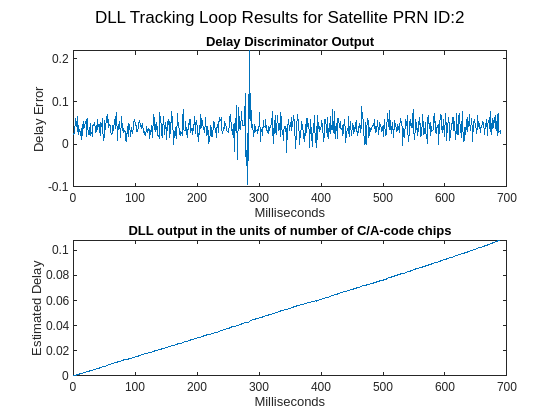
Plot the tracking loop results. The estimated phase error does not converge until the frequency locked loop converges. You can expect this behavior because the error in frequency causes an error in phase. Also, the outputs of PLL and FLL seem to change with time because of the changing Doppler shift.

if ShowVisualizations == 1
    for isat = 1 % To see tracking results for all the detected satellites by using above line
        groupTitle = ['Tracking Loop Results for Satellite PRN ID:', ...
            num2str(PRNIDsToSearch(isat))];

        figure

        % Plot the frequency discriminator output
        subplot(2,1,1)
        plot(accufqyerr(:,isat))
        xlabel('Milliseconds')
        ylabel('Frequency Error')
        title('Frequency Discriminator Output')

        % Plot the FLL output
        subplot(2,1,2)
        plot(accufqy(:,isat))
        xlabel('Milliseconds')
        ylabel('Estimated Frequency Offset')
        title('FLL Output')
        sgtitle(['FLL ' groupTitle])

        figure

        % Plot the phase discriminator output
        subplot(2,1,1)
        plot(accupherr(:,isat))
        xlabel('Milliseconds')
        ylabel('Phase Error')
        title('Phase Discriminator Output')

        % Plot the PLL output
        subplot(2,1,2)
        plot(accuph(:,isat))
        xlabel('Milliseconds')
        ylabel('Estimated Phase')
        title('PLL Output')
        sgtitle(['PLL ' groupTitle])

        figure

        % Plot the delay discriminator output
        subplot(2,1,1)
        plot(accudelayerr(:,isat))
        xlabel('Milliseconds')
        ylabel('Delay Error')
        title('Delay Discriminator Output')
        
        % Plot the DLL output
        subplot(2,1,2)
        plot(accudelay(:,isat))
        xlabel('Milliseconds')
        ylabel('Estimated Delay')
        title('DLL output in the units of number of C/A-code chips')
        sgtitle(['DLL ' groupTitle]) 
    end
end

Figure contains 2 axes objects and another object of type subplottext. Axes object 1 with title Frequency Discriminator Output, xlabel Milliseconds, ylabel Frequency Error contains an object of type line. Axes object 2 with title FLL Output, xlabel Milliseconds, ylabel Estimated Frequency Offset contains an object of type line.

Figure contains 2 axes objects and another object of type subplottext. Axes object 1 with title Phase Discriminator Output, xlabel Milliseconds, ylabel Phase Error contains an object of type line. Axes object 2 with title PLL Output, xlabel Milliseconds, ylabel Estimated Phase contains an object of type line.

Figure contains 2 axes objects and another object of type subplottext. Axes object 1 with title Delay Discriminator Output, xlabel Milliseconds, ylabel Delay Error contains an object of type line. Axes object 2 with title DLL output in the units of number of C/A-code chips, xlabel Milliseconds, ylabel Estimated Delay contains an object of type line.

After tracking, plot the constellation of the signal.

if ShowVisualizations == 1
    rxconstellation = comm.ConstellationDiagram(1,"ShowReferenceConstellation",false);
    demodsamples = accuintegwave(301:end,:)/rms(accuintegwave(:));
    if ~isempty(demodsamples)
        rxconstellation(demodsamples(:));
    end
end 

If constellation points appear at the center in a constellation diagram, they correspond to the false detection of a satellite from the acquisition algorithm.

Further Exploration

This example has shown you how to perform GPS signal acquisition and tracking for four GPS satellites and using an ADALM-Pluto radio for over-the-air transmission. To explore further, try these variations:

  • Increase the number of visible GPS satellites and observe the results. Initialize the Doppler, SNR, and delay appropriately.

  • Simulate real-time GPS signal, by scaling the GPS signal amplitude below the noise floor, and check the acquisition and tracking using the ADALM-PLUTO radio.

  • Perform position estimation with the SDR device. You may need to use two PlutoSDR devices (one for transmission and another for reception). For more information on position estimation, see the End-to-End GPS Legacy Navigation Receiver Using C/A-Code example.

Appendix

This example uses these data and helper files:

References

[1] IS-GPS-200, Rev: L. NAVSTAR GPS Space Segment/Navigation User Segment Interfaces. May 14, 2020; Code Ident: 66RP1.